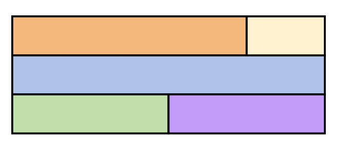
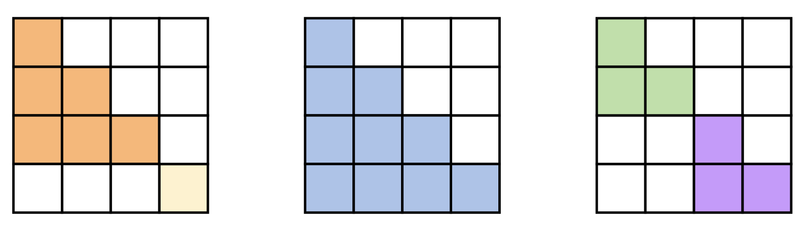
To first approximation, LLM training consists of three types of matrix muliplications (GEMMs): forward matmul, activation gradient matmul, and weight gradient matmul. On token level, the GEMM reduces to matrix vector product: weight times activation . Suppose and , then takes multiply and accumulation operations where is the number of weight parameters. One forward and two backwards GEMMs thus account for operations per token. This scales linearly with the number of GEMMs in an LLM, so a back-of-envelop calculation says where is the number of active model parameters (in MoE model, not all parameters are active for every token). Thus for an MoE with experts of which are activated per token
We now compute the average communication volume per GPU participating in the dispatch phase of expert parallelism. Let be the total number of experts in a MoE model, in which each token is routed to distinct experts. Suppose each of the experts is equally likely to be chosen. Fix a GPU holding experts. A token at this GPU chooses experts, of which are located on other GPUs. Thus follows a hypergeometric distribution distribution and Let us make a further assumption that each GPU holds the same number of experts, i.e. the number of expert parallel GPUs is so that Let the token dimension be , sequence length at our fixed GPU is , and the datatype precision is bytes-per-float. The expectation of the communication volume in bytes for this single GPU at dispatch phase is Likewise the variance of can be computed from the variance of In reality one might additionally send block-scale factors in addition to the tokens, and the inputs are often batched. The corresponding modifications from the foregoing should be straight forward. During the combine phase tokens are routed back in the opposite direction of dispatch phase so the magnitude of communication is identical.
We now analyze MoE backward communication. For simplicity we analyze this at the token level. Let be the parametrized mappings implemented by the experts (weights in , tokens in ) . Suppose each token in the vocabulary activates a -subset of the experts and is the remainder of the forward pass after the MoE until the loss is computed. Note, we sometimes write for simplicity, in all such usecases, expert weights can be effectively treated as constant. By the chain rule, the expert weights are updated by for where we write to mean the derivative with respect to and will mean the derivative with respect to . Thus MoE weight gradient computation requires dispatching the activation gradient to the activated experts. Knowing will also enable each expert to compute the activation gradients . These will enable us to compute the activation gradients Since the derivative is a linear map, the composition can be distributed over the sum, so that in reality this activation gradient can be computed through a combine operation. Communication occurs for all non GPU-local experts in the reverse direction of forward dispatch and combine, where forward combine becomes backward dispatch, and forward dispatch becomes backward combine. Thus the sequence level communication volume for each of backwards dispatch and combine is also
MoE Layer
Click to enlarge
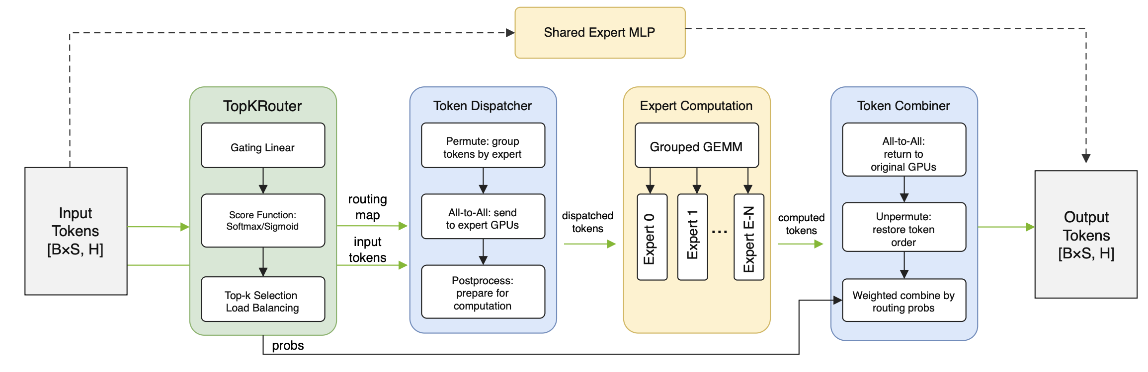
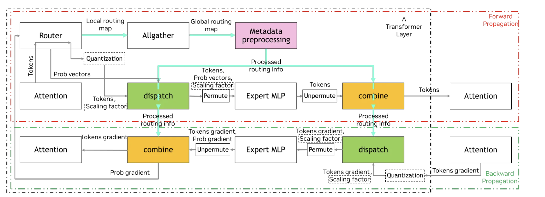
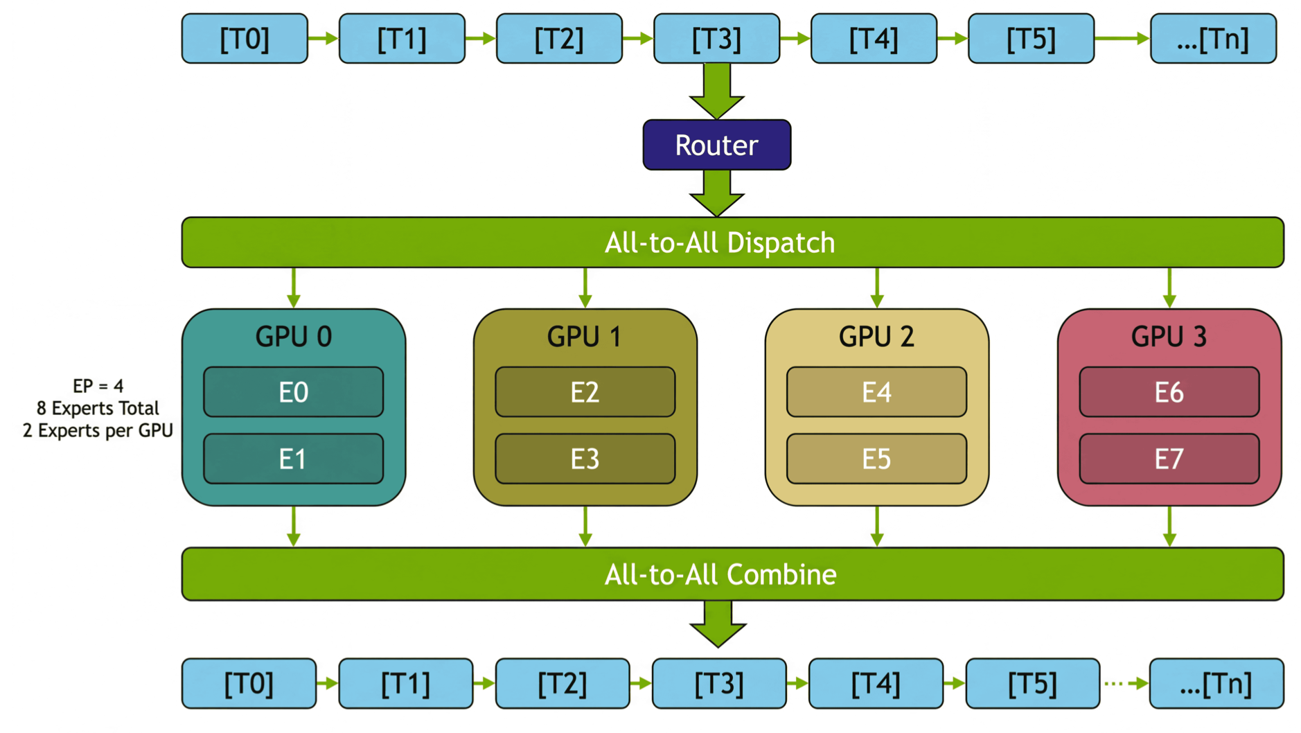
Expert selection, token dispatch, expert computation, and token combine stages of MoE layer forward pass (Megatron paper). Two practical notes are that (1) tokens are permuted before dispatch, and inversely permuted after combine and (2) expert router uses high precision FP for numerical stabillity of opertions like exponentiation in softmax, for example, and possibly Top- selection.
Load balancing mechanisms can be applied at three locations: router logits (z-loss, Sinkhorn), token probabilities (expert bias), and Tok- selection (global/micro batch and sequence auxilary loss).
Dispatch and combine can use different backends, from DeepEP, HybridEP, to collectives like All-to-All (every GPU sends data to and receives data from every peer) and AllGather+ReduceScatter (redundant). Approaches such as DeepEP and HybridEP implement more nuanced optimization than directly using the fundamental communication collectives.
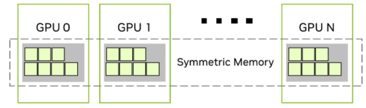
Communication across GPUs is facilitated by the set of CUDA virtual memory managment APIs. Each GPU allocates memory, and generates a pointer that is shared with participating peer GPUs so that each peer GPU maps remote memory of to the virtual memory of . The virtual memory space of corresponding to the set of all remote memory of all participating GPUs is called the symmetric memory space and can read from and write to the symmetric memory using the same programming interface (instructions and APIs) in kernels in the same way does its physical global memory.
Click to enlarge
The symmetric memory read and write are physically mediated by NVLink (TRT blog)
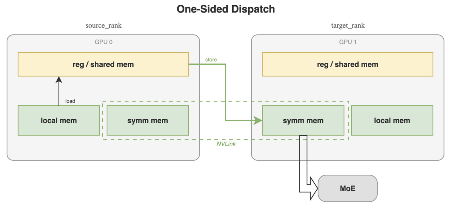
Click to enlarge
Tracing data movement during dispatch (TRT blog)
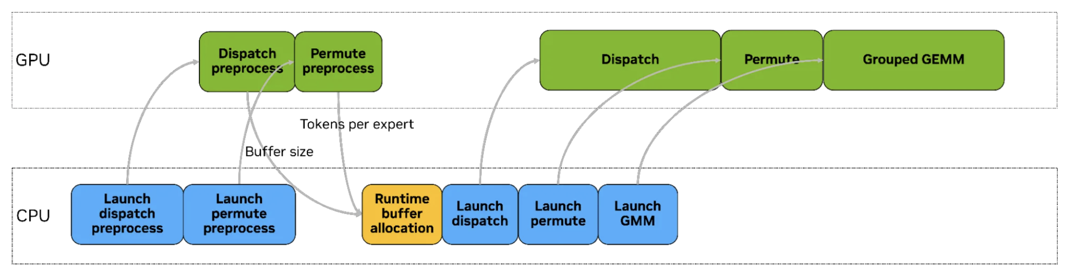
The kernel design of Hybrid-EP kernels are as follows.
Click to enlarge
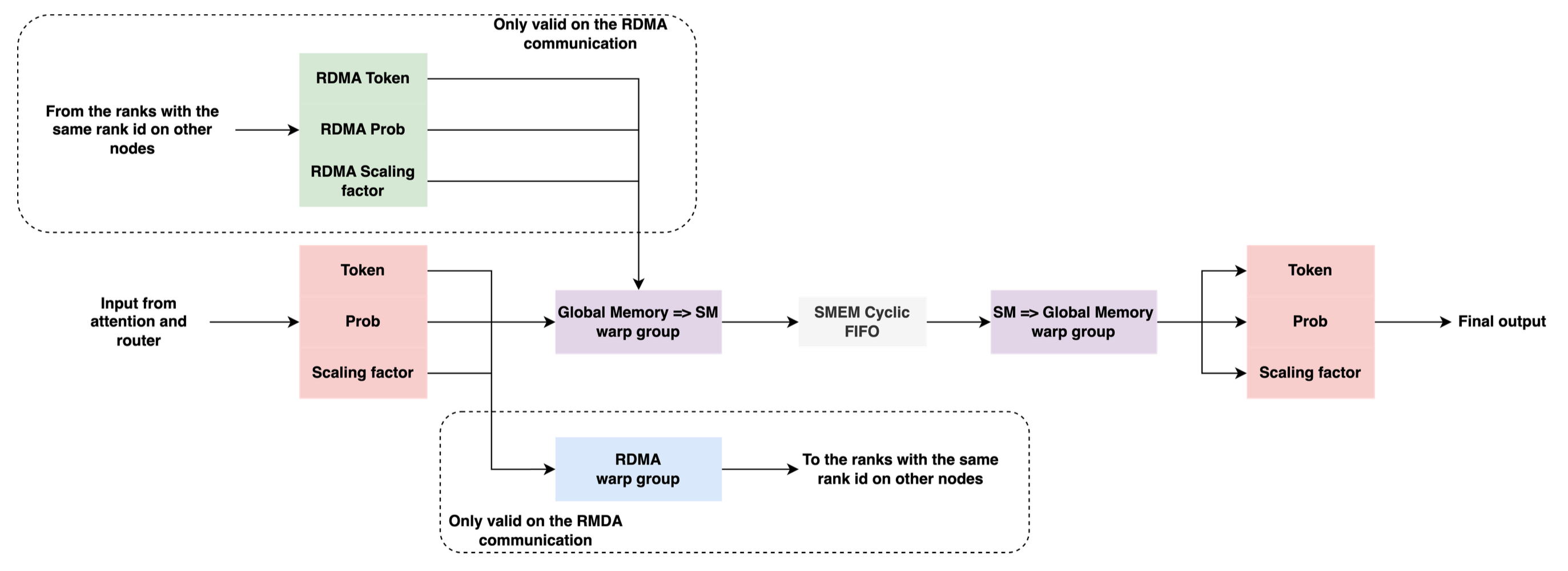
HybridEP dispatch kernel design (Megatron paper).
An interesting feature of the dispatch kernel is that during cross node communication, a remote direct memory access warp group exchanges data between GPUs of the same local rank on different nodes, and then forwards within the node via NVLink.
Click to enlarge
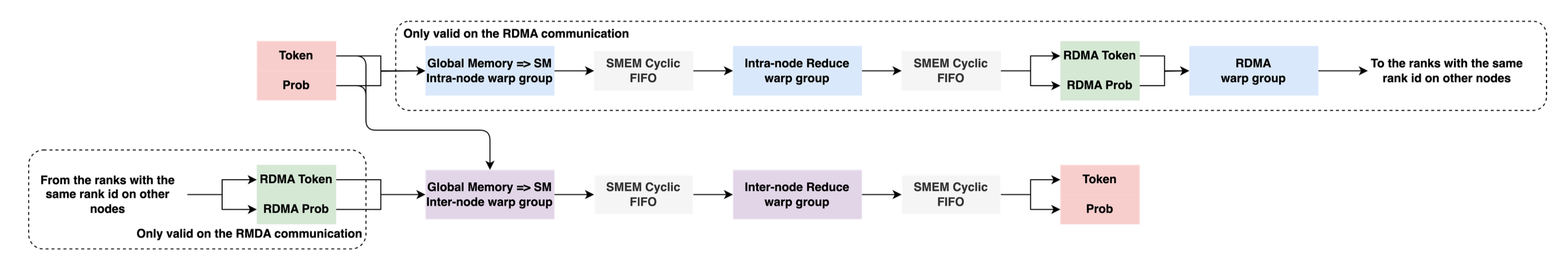
HybridEP combine kernel design (Megatron paper).
For the combine kernel, communication and reduction (i.e. linear combination of expert outputs during forward, or activation gradients during backward) are fused. The reduction is performed in two stages, first cross node reduction, followed by within node reduction.
Click to enlarge
HybridEP forward and backward (HybridEP blog)
Click to enlarge
Overlaping forward and backward (Megatron paper)
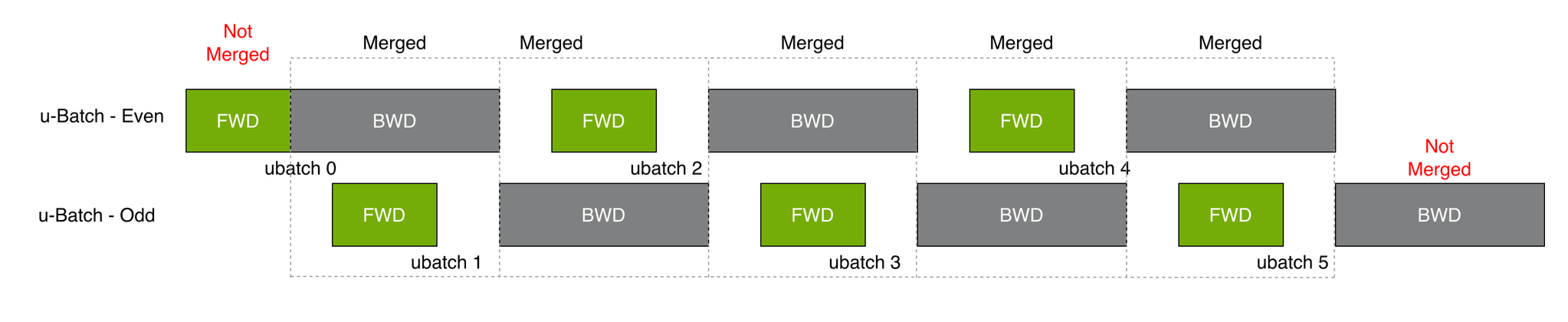
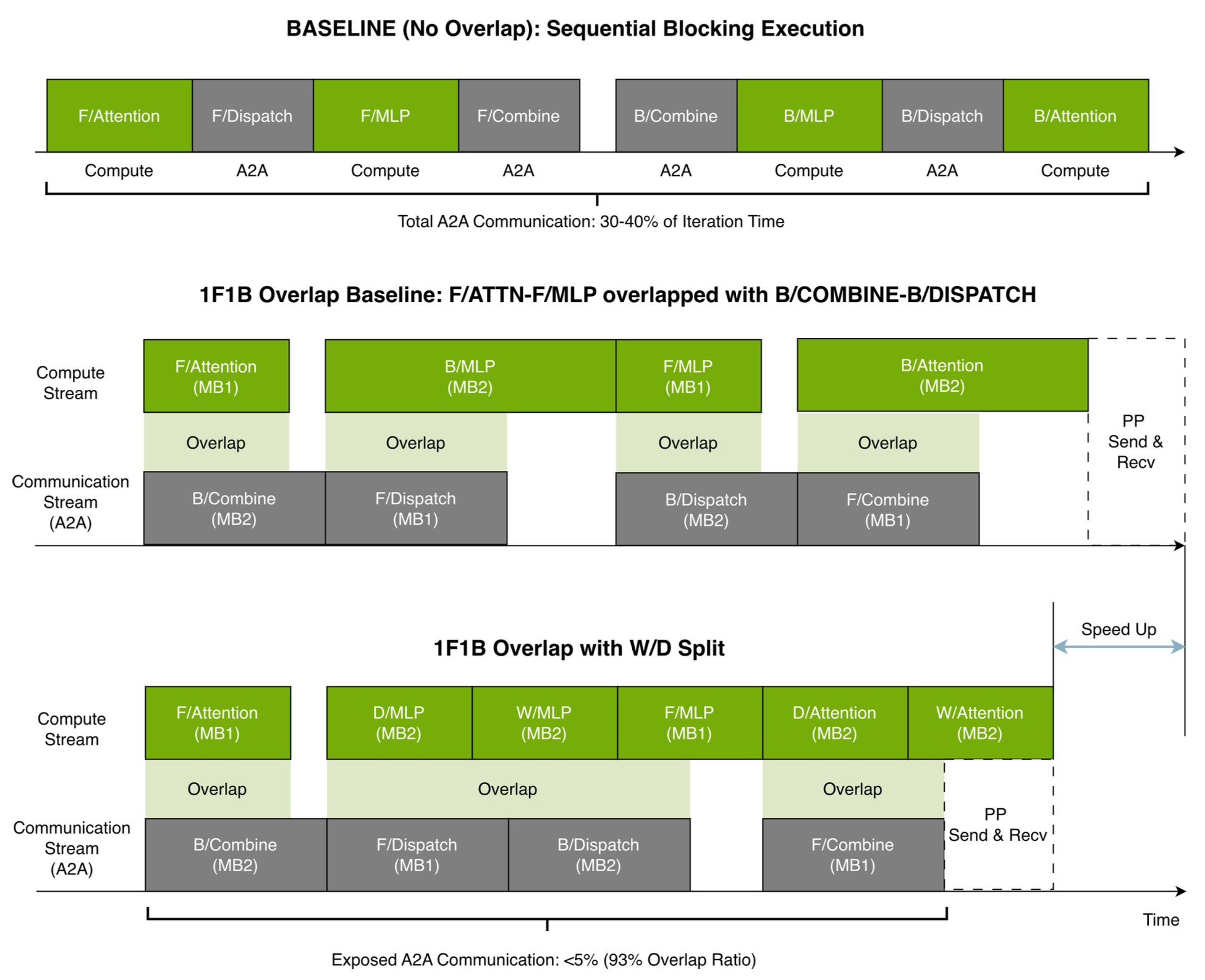
In order to hide communication latency, one can simultaneously execute a forward and backward on a pair of microbatches. Optimization include using a pair of CUDA streams, one for computation (attention, MLP), and another for communication (token dispatch and combine). Let us zoom in the forward and backward:
Click to enlarge
Forward and backward comparison (top) no overlap (middle) simultaneously excute a forward and backward pair (bottom) smarter scheduling of activation gradient and weight gradient computation (Megatron paper)
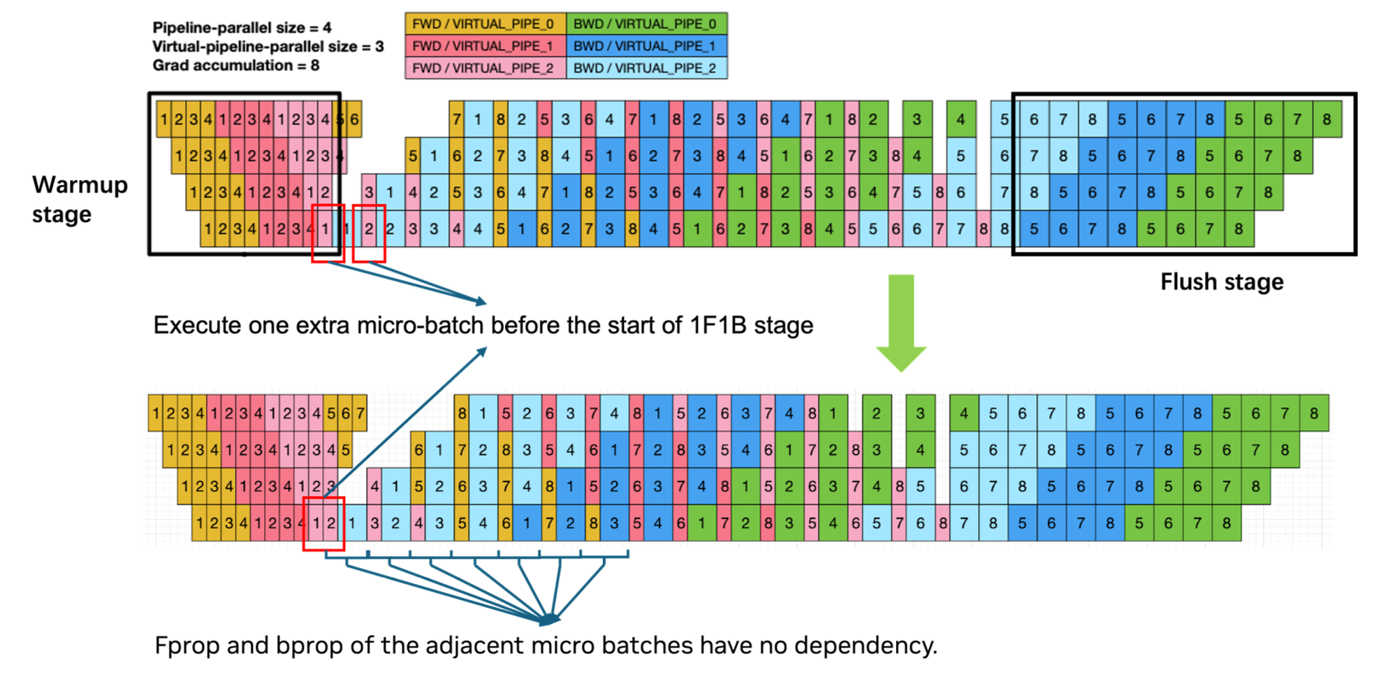
The above idea can be scaled up as follows, in which each row is associated with a GPU (Pipeline parallel size PP=4, virtual pipeline size VPP=3), adjacent forward and backward are overlapped, there are gradient accumulations (hence microbatches) before weight update. The execution is prefaced by a warmup stage, followed by 1F1B, and appended by a flush stage.
Parallelism is a mechanism for managing memory and improving arithmetic intensity. Parallel is effective when communication can be hidden by computation time. Recall the common forms of parallelisms for dense transformers.
Context parallel partitions the input along the sequence direction to be processed by different GPUs. Communication occurs for attention operation (exchange of KV cache), which crosses chunk boundaries. CP is particularly useful for the long context regime. In pretraining the sequence length is fixed, but in reinforcement learning, the variable length of rollouts is a challenge. This is mitigated by a variation of CP called dynamic context parallel in which CP size is adaptively determined based on microbatch sequence length.
Tensor parallel partitions matrices along the hidden dimension. Communication occurs to combine partial results. Tensor parallel is effective in the regime when matrices are large to justify communication. Large matrices in products can benefit from TP.
Pipeline parallel shards different layers across GPUs, communication takes place one layer chunk and the next. Pipeline bubbles is a main source of inefficiency, and can be alleviated by clever scheduling of microbatches.
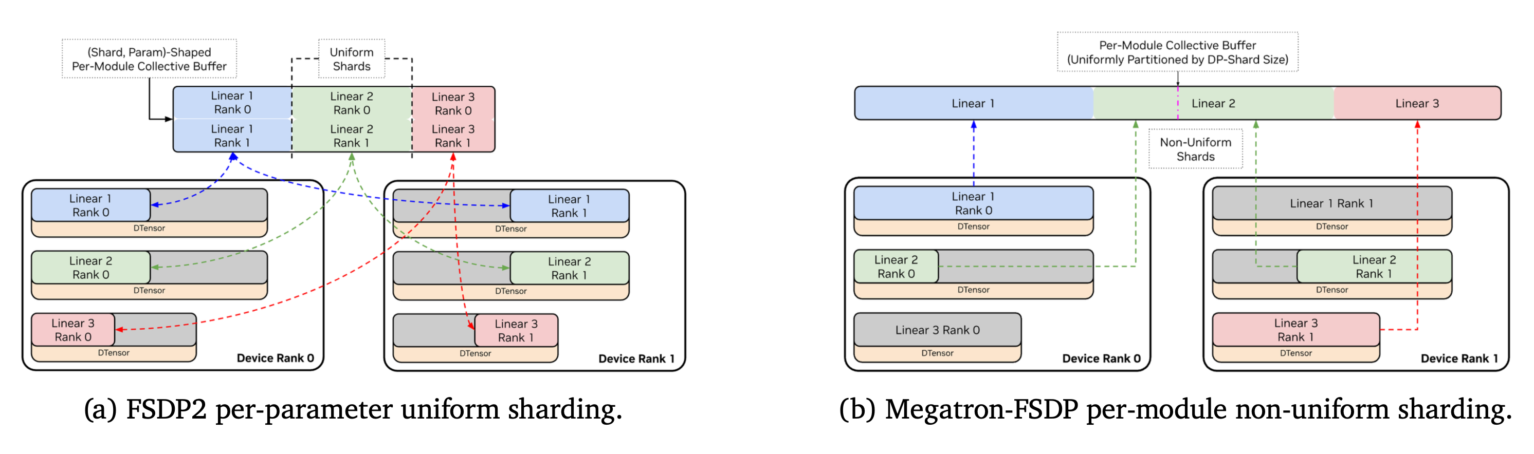
Data parallel shard data across model replicas, communication occurs for gradient all-reduce. Fully sharded data parallel is used to shard optmizer states and gradient model weights so that full tensors are materialized (communication required) only when needed, and disassembled immediately afterwards. One notable variation in FSDP implementation is the Megatron FSDP, in which all parameters in a layer are flattened and concatenated. In Megatron FSDP shard boundaries align with communication buffer so that zero-copy collectives can be used, and the streaming multiprocessor usage for communication kernels drops.In this variation however, tensor might be non-uniformly sharded.
Click to enlarge
Megatron FSDP (Megatron paper)
To scale MoE model training, expert parallel is used, in which expert FFNs are sharded across GPUs. The communication volume scales with as we saw earlier with .
In pratice, different parallelisms are used for the attention and for MoE layers.
Click to enlarge
Expert parallel (Megatron paper)
Memory Efficiency
Managing memory is a priority to ensure training runs, but more memory also enables additional optimization, for instance larger batch sizes to increase compute intensity and hide communication latency.
Activation memory is often the dominant memory consumer in MoE training. Activation memory scales both with input (batch size, sequence length, hidden size) as well as with architecture (layer depth, the number of activated experts per token). Techniques for reducing memory include FSDP (mentioned above), low precision data types, activation recomputation, activation offloading, each coming with its own tradeoffs and subtleties.
Take activation recomputation as a case study. On approach is to save layer inputs only, and recompute activations throughout the layer when needed, this is sometimes called full recomputation. If activation recomputation is applied without care, and full recomputation is applied to the MoE layers, then expert communication can be duplicated 🙀. A better approach would targets select activtion to be recomputed, especially when the memory savings outweights computation costs incurred in recomputation. For example, one can recompute LayerNorm, while offloading attention activations to CPU. Thus in the design of training framework, one require a mechanism for each computation to specify memory strategy to manage the activation produced by that computation. When activation recomputation is activated, we need to promptly release activations that will be recomputed.
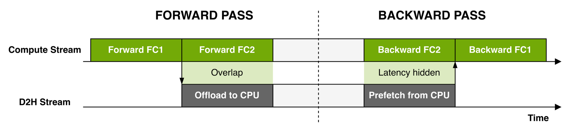
Activation can also be offloaded to CPU memory during forward pass, then fetched during backward pass. Efficiency is gained through overlapping GPU computation with device-to-host data transfer in distinct CUDA streams.
Click to enlarge
Overlapping computation with device-host communication (Megatron paper) The edge case occurs at the first and last layer, when either activation is not yet generated, or when activation is immediately need for loss computation, therefore it is not offloaded, but the communication stream in fact prefetches activation for the second last layer. During backward, activation prefetching must be coordinated, since pretching too many activations can spike the memory, defeating the purpose of activation offloading.
Another method is rearranging the math to reduce activation, for example in the FFN, the scalars (probabilities) are applied after inner activation function. To see an example, take the earlier MoE example with experts implemented with matrices , , probabilities , and activation function We focus on one expert and omit its subscript. Computing the FFN in this order requires activation to be kept in memory to compute . But if we rearrange the order of computation then we no longer need to save the activation to compute . In the latter formulation, to compute loss gradient with respect to we can recompute from saved activation (which is saved to compute ).
Beyond activation memory, optimizer states also occupies much memory, storing first and second moments for each model parameter. Precision aware optimizerdecouples storage and precision requirements, in which storage occurs at low precision, but computation is recasted to a high precision (e.g. FP32) with optimizer kernels, in order to maintain numerical stability. Whenever optimizer states and master weights are inactive, they are offloaded to the CPU until they are needed again.
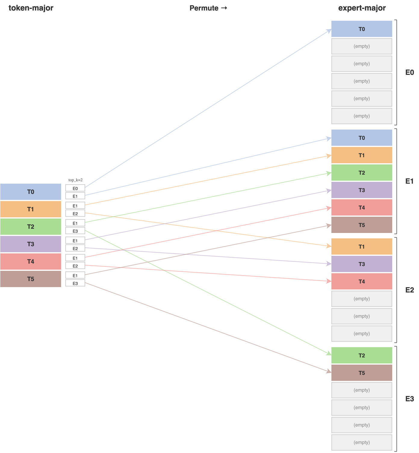
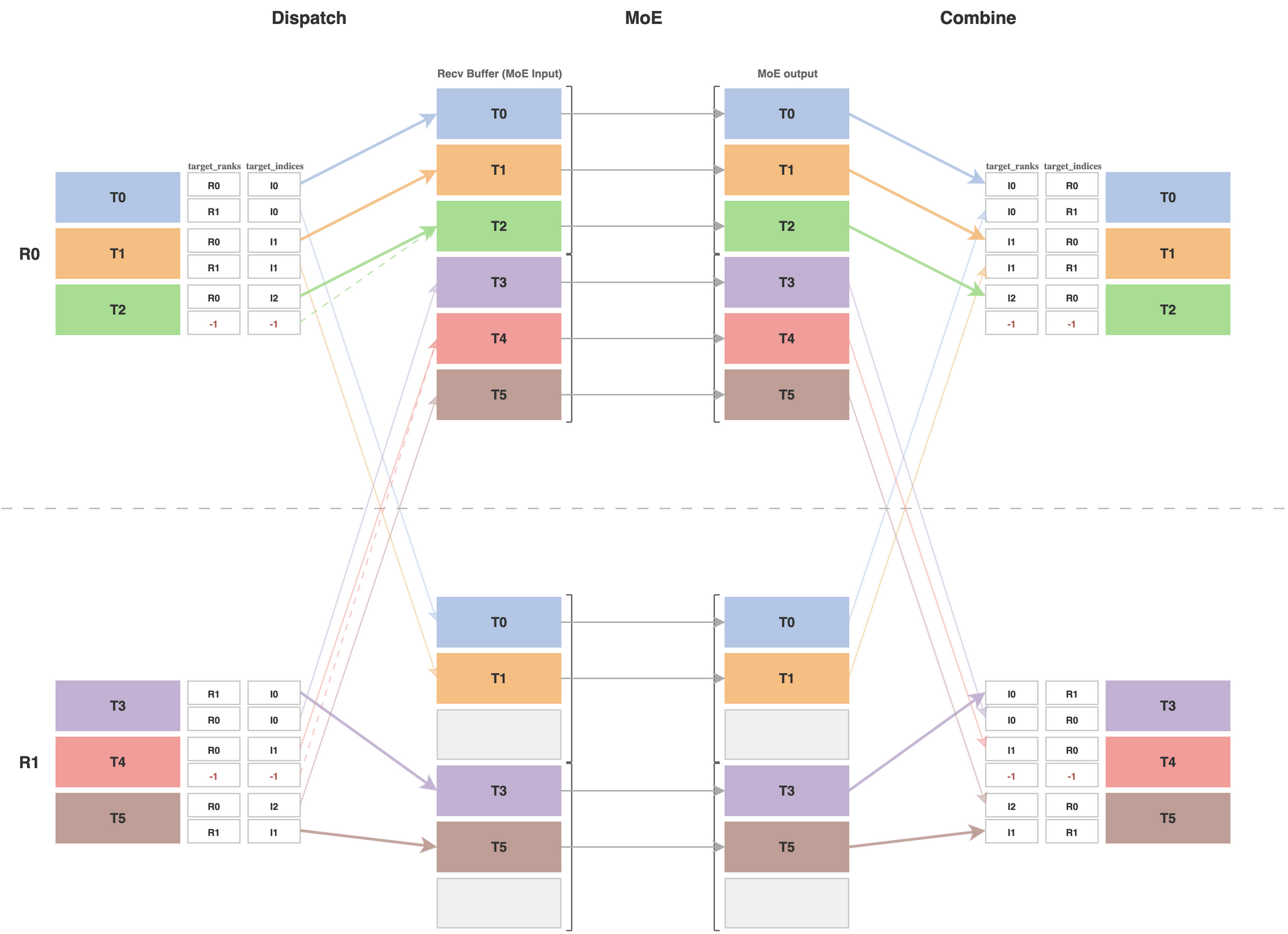
Training also requires various buffers. Instead of allocating worst case buffers everytime, instead maintain a single persistent buffer together with a number of smaller (average case buffers). This technique is the paged stashing mentioned in the Megatron paper. Another buffer memory optimization from TensorRT performs deduplication for any token that gets sent multiple times to experts located on the same GPU. The strategy is that during dispatch phase, each expert parallel rank allocates not expert-major but instead token-major here the omitted dimension include hidden dimension, scale factor (if using quantization) and possibly other metadata. The memory buffer saving is visualized as follows
Click to enlarge
Memory optimization from using token major receive buffers (TRT blog)
Click to enlarge
Dispatch and combine with TRT deduplication optimization, -1 indicates same token routed to experts on same rank (TRT blog)
Compute Efficiency
The main strategies are kernel fusion, CUDA graph, and load balancing (MoE specific).
A barrier to compute efficiency originate from the small GEMM size in MoE layers (especially fine-grained MoEs) which incompletely uses tensor core. Kernel fusion of a large number of small GEMM kernel lanuches into a large grouped GEMM kernel help improve compute efficiency. GEMMs can also be computed in low precision to increase throughput while reducing data movement, in these cases quantization is required. A kernel fusion opportunity for this is to quanitze multiple tensors at once, this fusion leads to what is called a grouped quantization kernel. Yet another type of kernels fuse together quantization, GEMM, and activation.
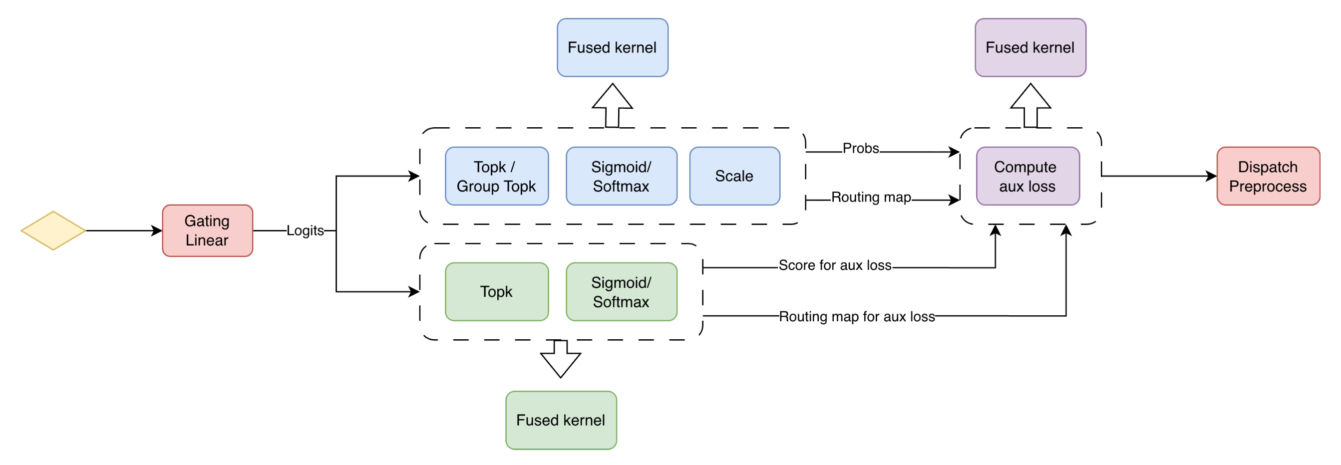
Grouped GEMMs require permutation operations, these are optimized with kernel fusion. Router and auxiliary loss are also fused:
Click to enlarge
Kernel fusions for router and auxiliary loss computations (Megatron paper)
Kernel lanuches incurs CPU overheads that can result in bubbles in GPU execution timeline. CUDA graph can be used to elinminate the bubbles provided kernels are static and have known problem sizes. CUDA graphs are not available for dynamic problem sizes and control flow. Due to the variable number of tokens that gets assigned to each expert, the expert GEMMs, dispatch and combine do not have predetermined problem shapes. Constant sizes can be enforced by assigning determined sizes to each expert and dropping excessive tokens or padding to the set size if an expert received less than determined number of tokens.
If we choose a dropless MoE, then we can partition the transformer operations into those with (resp without) predetermined problem sizes. Then CUDA graph is applied to those with predetermined sizes only. There are nuances to using CUDA with parallelism, for instance, in pipeline parallel, each microbatch has its own CUDA graph. Dynamic problem sizes are often known by synchronizing with the CPU host, creating inefficiencies, this is addressible by using GPU device initiated kernels.
In MoE training some experts may be receive more tokens than others, causing load imbalance. One solution replicates overloaded experts. This has a tradeoff against communication efficiency. The bin-packing algorithm is used to determine which experts should be cloned, together with its placement among GPUs.
Mixed Precision
While low precision increase computation throuput, sensitive operations need high precision. High precision operation include MoE routing, embedding, output, main gradient, master weight, optimizer states. Low precision operations include GEMMs, storage for activation memory. The tradeoff include quantization overheads, which can be addressed by kernel fusion.
Low precision such as NVFP4 require nontrivial receipes and careful optimization of such operations as random Hadamard transform (reduce outlier), 2D scaling (make block scaling transpose friendly, useful for backwards gradient computation), stochastic rounding (mitigate rounding bias).
When low precision weights are used, usually a higher precision weight copy (sometimes referred to as master weight) is maintained, for which quantization kernel is needed.
Long Context Training
Training requires taming compute, memory, and communication. Optimized GEMM and attention kernels such as FlashAttention places the emphasis on memory (epecially activation memory), and communication.
Long context training activation memory can be managed mainly by a combination of CP x TP. The previously introduced CPU offloading of optimizer states and recomputation are applicable but less effective than CP x TP.
Variable Context Training
In reinforcement learning, bin packing algorithm is used to pack variable length sequences into the context window bins.
Click to enlarge
Batch of 3 packing sequences
Accordingly the causal masks applied at scaled dot product attention is modified to avoid attending cross sequence boundaries.
Click to enlarge
Attention masks corresponding to each of the 3 packed sequences
Loss computation also needs to be modified accordingly as a result of sequence packing.